---
title: "View Introspection Network (VIN) on EVL"
format: html
---
# Scope
This page documents the current **VIN** implementation in `oracle_rri/oracle_rri/vin/`: a lightweight **RRI predictor head** trained on top of a **frozen EVL backbone** (EFM3D). It replaces expensive oracle computations at inference time by predicting **Relative Reconstruction Improvement (RRI)** for a set of candidate poses.
References:
- Paper summary: [VIN-NBV](../literature/vin_nbv.qmd)
- EFM3D/EVL implementation map: [EFM3D Implementation Index](../ext-impl/efm3d_implementation.qmd)
- External EVL docs: [Project Aria Tools — EVL](https://facebookresearch.github.io/projectaria_tools/docs/open_models/evl)
- External code: [facebookresearch/efm3d](https://github.com/facebookresearch/efm3d)
- CORAL ordinal regression (implementation): [coral-pytorch](https://raschka-research-group.github.io/coral-pytorch/) ([GitHub](https://github.com/Raschka-research-group/coral-pytorch))
- Oracle label pipeline: [RRI computation](rri_computation.qmd) and `oracle_rri/oracle_rri/pipelines/oracle_rri_labeler.py`
- VIN implementation: `oracle_rri/oracle_rri/vin/model.py` (`VinModel`), `oracle_rri/oracle_rri/vin/model_v2.py` (`VinModelV2`), and `oracle_rri/oracle_rri/lightning/lit_module.py` (`VinLightningModule.summarize_vin`)
- Optional trajectory encoder: `oracle_rri/oracle_rri/vin/traj_encoder.py` (`TrajectoryEncoder`) for R6D+LFF encoding of `EfmTrajectoryView.t_world_rig`. In VIN v2, per-frame trajectory encodings are transformed into the reference rig frame and can be cross-attended by candidate pose embeddings.
# Problem statement
Given:
- the current state encoded as a raw EFM snippet dict `efm: dict[str, Any]` (see `oracle_rri.data.EfmSnippetView.efm`), and
- a set of candidate next viewpoints as poses $T_{\text{world}\leftarrow\text{cam}_i}$ (`PoseTW`, **world←camera**) with $N$ candidates,
predict per-candidate scores $\widehat{\text{RRI}}(q_i)$ such that selecting $\arg\max_i \widehat{\text{RRI}}(q_i)$ approximates selecting $\arg\max_i \text{RRI}(q_i)$ computed by the oracle.
# EVL backbone recap
EVL (Egocentric Voxel Lifting) processes the snippet and produces a **voxel-aligned 3D representation**. Architecturally (simplified), it follows:
```{mermaid}
flowchart LR
    A["EFM snippet dict<br/>(images, poses, calib, semidense)"]
    A --> B["2D backbone<br/>(DinoV2 / video backbone)"]
    B --> C["Lifter<br/>(voxel grid + evidence<br/>+ T_world_voxel)"]
    C --> D["3D neck<br/>(feature refinement)"]
    D --> E["Heads<br/>(occupancy + OBB detection)"]
    C --> F["VIN head<br/>(ours)"]
    E --> F
    F --> G["CORAL logits<br/>(ordinal RRI bins)"]
```
For VIN we want a compact, information-rich scene embedding that is (a) available for every snippet, (b) stable across training/inference, and (c) cheap to query for many candidates. For the current **minimal VIN v0.1**, we therefore prioritize **low-dimensional head/evidence volumes** over heavy neck features.
The rich **3D neck feature volumes** can be exposed for ablations. In `external/efm3d/efm3d/model/evl.py`, they are created right before the occupancy / OBB heads:
- `out["neck/occ_feat"] = neck_feats1`
- `out["neck/obb_feat"] = neck_feats2`
Our stable “feature contract” is implemented by `oracle_rri/oracle_rri/vin/backbone_evl.py` (`EvlBackbone`). Minimal VIN uses:
- `occ_pr` (occupancy head output)
- `voxel/occ_input` (occupied evidence)
- `voxel/counts` (coverage)
- `voxel/T_world_voxel`, `voxel_extent` (coordinate contract)
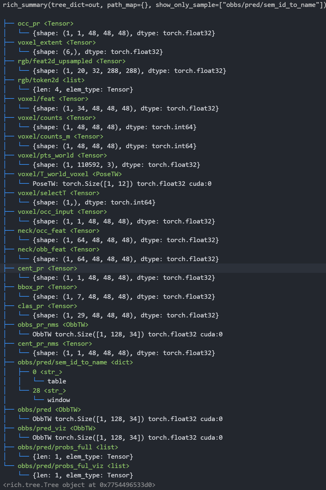
`EvlBackbone` can optionally expose richer tensors (neck features, decoded OBBs) for future variants:
```
├── occ_pr <Tensor>
│   └── {shape: (1, 1, 48, 48, 48), dtype: torch.float32}
├── voxel_extent <Tensor>
│   └── {shape: (6,), dtype: torch.float32}
├── rgb/feat2d_upsampled <Tensor>
│   └── {shape: (1, 20, 32, 288, 288), dtype: torch.float32}
├── rgb/token2d <list>
│   └── {len: 4, elem_type: Tensor}
├── voxel/feat <Tensor>
│   └── {shape: (1, 34, 48, 48, 48), dtype: torch.float32}
├── voxel/counts <Tensor>
│   └── {shape: (1, 48, 48, 48), dtype: torch.int64}
├── voxel/counts_m <Tensor>
│   └── {shape: (1, 48, 48, 48), dtype: torch.int64}
├── voxel/pts_world <Tensor>
│   └── {shape: (1, 110592, 3), dtype: torch.float32}
├── voxel/T_world_voxel <PoseTW>
│   └── PoseTW: torch.Size([1, 12]) torch.float32 cuda:0
├── voxel/selectT <Tensor>
│   └── {shape: (1,), dtype: torch.int64}
├── voxel/occ_input <Tensor>
│   └── {shape: (1, 1, 48, 48, 48), dtype: torch.float32}
├── neck/occ_feat <Tensor>
│   └── {shape: (1, 64, 48, 48, 48), dtype: torch.float32}
├── neck/obb_feat <Tensor>
│   └── {shape: (1, 64, 48, 48, 48), dtype: torch.float32}
├── cent_pr <Tensor>
│   └── {shape: (1, 1, 48, 48, 48), dtype: torch.float32}
├── bbox_pr <Tensor>
│   └── {shape: (1, 7, 48, 48, 48), dtype: torch.float32}
├── clas_pr <Tensor>
│   └── {shape: (1, 29, 48, 48, 48), dtype: torch.float32}
├── obbs_pr_nms <ObbTW>
│   └── ObbTW torch.Size([1, 128, 34]) torch.float32 cuda:0
├── cent_pr_nms <Tensor>
│   └── {shape: (1, 1, 48, 48, 48), dtype: torch.float32}
├── obbs/pred/sem_id_to_name <dict>
│   ├── 0 <str_>
│   │   └── table
│   └── 28 <str_>
│       └── window
├── obbs/pred <ObbTW>
│   └── ObbTW torch.Size([1, 128, 34]) torch.float32 cuda:0
├── obbs/pred_viz <ObbTW>
│   └── ObbTW torch.Size([1, 128, 34]) torch.float32 cuda:0
├── obbs/pred/probs_full <list>
│   └── {len: 1, elem_type: Tensor}
└── obbs/pred/probs_ful_viz <list>
    └── {len: 1, elem_type: Tensor}
```
## Key-by-key explanation and “should VIN use it?”
### A) Core voxel geometry / coordinate contract
#### `voxel/T_world_voxel` — `PoseTW` (B, 12)
**What it is:** The pose of the voxel grid in world coordinates (**world←voxel**). The voxel grid is anchored to the **last frame** of the snippet and gravity-aligned (roll/pitch ≈ 0; yaw-only). ([GitHub][1])
**Use for VIN?** **Must-use.** You need it to map candidate-frustum 3D sample points (world) into voxel coordinates for trilinear sampling.
#### `voxel_extent` — `(6,)`
**What it is:** `[x_min, x_max, y_min, y_max, z_min, z_max]` defining the voxel grid’s metric bounds **in the voxel frame** (meters). EVL passes this around explicitly. ([GitHub][2])
**Use for VIN?** **Must-use.** Required to normalize voxel coordinates and implement valid masks for sampling.
**Debug note (common confusion):** the EVL voxel grid is intentionally **local and fixed-size** (default in our setup is a 4 m cube: `[-2, 2] × [0, 4] × [-2, 2]`). This means the voxel bounds can look *much smaller* than the snippet’s semi-dense cloud or crop bounds. That is expected: EVL only lifts a local volume anchored at `voxel/selectT` rather than the full scene. The size is configured in `external/efm3d/efm3d/config/evl_inf_desktop.yaml`. ([GitHub][3])
#### `voxel/pts_world` — `(B, D*H*W, 3)` (here 110592 = 48³)
**What it is:** The world coordinates of every voxel center (a flattened voxel grid). It’s generated from `voxel_extent` and `T_world_voxel`. ([GitHub][1])
**Use for VIN?** **Usually no.** It’s redundant (you can generate the same points on demand). Only useful for debugging/visualization or if you want a one-time precomputed voxel-center point cloud.
#### `voxel/selectT` — `(B,)` int
**What it is:** The selected time index used to anchor the voxel grid (by default `T-1`). ([GitHub][1])
**Use for VIN?** **No (training), yes (debug).** You typically only need `T_world_voxel` directly.
---
### B) Observation evidence injected into 3D (high value for NBV/RRI)
#### `voxel/counts` — `(B, D, H, W)` int64
**What it is:** For each voxel, how many snippet frames/streams produced a **valid projection** into the image during lifting. It is computed as a sum over valid projection masks. ([GitHub][1])
**Use for VIN?** **Yes (strongly recommended).** This is a direct proxy for *coverage / observation density* inside EVL’s voxel volume.
**Practical note (current VIN):** We normalize counts **per snippet** using the maximum count inside the voxel volume, either
linearly or with a `log1p` compression (default). Concretely, with $c(\mathbf{v}) \in \mathbb{N}$:
$$
c_{\max}=\max_{\mathbf{v}} c(\mathbf{v}),\qquad
\text{counts\_norm}(\mathbf{v})=
\begin{cases}
\dfrac{\log(1+c(\mathbf{v}))}{\log(1+c_{\max})} & \texttt{counts\_norm\_mode="log1p"}\\[6pt]
\dfrac{c(\mathbf{v})}{c_{\max}} & \texttt{counts\_norm\_mode="linear"}
\end{cases}
$$
#### `voxel/counts_m` — `(B, D, H, W)` int64
**What it is:** A “masked/debug” variant of the counts (EVL explicitly says it’s passed for debugging). ([GitHub][1])
**Use for VIN?** **No for learning**, unless you’ve verified it’s identical to what you want. Prefer `voxel/counts` + explicit masking logic in your VIN.
#### `voxel/occ_input` — `(B, 1, D, H, W)` float (mask)
**What it is:** A binary occupancy mask derived from the input 3D points (semi-dense/GT points in the batch): EVL voxelizes the point cloud and turns voxels with any points into `1.0`. ([GitHub][1])
**Use for VIN?** **Yes.** This is extremely aligned with the oracle’s “current reconstruction” (semi-dense points), and it helps predict where RRI can still improve.
#### `voxel/feat` — `(B, F, D, H, W)` (here F=34)
**What it is:** The raw lifted voxel feature volume **before** the neck. It is:
* lifted + aggregated 2D features (here 32 channels),
* concatenated with `point_masks` and `free_masks` (2 extra channels). ([GitHub][1])
**Use for VIN?**
**Not for minimal VIN v0.1.** It’s a fat tensor that’s less refined than the head outputs, and it adds semantics that we have not validated across EVL configs/checkpoints. We intentionally keep the current scorer head limited to `occ_pr`, `occ_input`, and `counts_norm`.
---
### C) 3D neck features (rich, but heavier)
#### `neck/occ_feat` — `(B, 64, D, H, W)`
**What it is:** The refined 3D feature volume right before the occupancy head. EVL stores it explicitly. ([GitHub][2])
**Use for VIN?** **Optional.** If you want “maximum information” from EVL, this is the most stable attachment point. But it’s heavier than head outputs.
If you use it: **compress channels** with a 1×1×1 conv (e.g., 64 → 16/32) before any pooling/sampling.
#### `neck/obb_feat` — `(B, 64, D, H, W)`
**What it is:** Refined 3D features right before the OBB detection head. ([GitHub][2])
**Use for VIN?** **Optional / future entity-aware.** For pure geometry-RRI, you can omit it initially.
---
### D) Occupancy head output (surface reconstruction head)
#### `occ_pr` — `(B, 1, D, H, W)` float32
**What it is:** The **occupancy prediction** after sigmoid: `occ_pr = sigmoid(occ_logits)`. ([GitHub][2]) In VIN we
also support treating `occ_pr` as logits via `VinModelConfig.occ_pr_is_logits` in case an EVL variant exposes logits.
**Use for VIN?** **Yes.** This is the single most sensible “head output” for an RRI predictor.
How to use:
* Global pooling (mean/max) for a snippet descriptor.
* Candidate-conditioned **frustum sampling** (sample voxels along candidate view rays) to estimate how much *unknown/occupied* structure lies ahead.
---
### E) OBB detection head raw grids (dense, per-voxel predictions)
These are the “dense detection maps” before decoding into box lists.
#### `cent_pr` — `(B, 1, D, H, W)`
**What it is:** Center probability map after sigmoid: `cent_pr = sigmoid(cent_logits)`. ([GitHub][2])
**Use for VIN?** **Maybe.** It encodes “objectness / box centers.”
* If your RRI is purely geometric, it’s optional.
* If you want an **object-biased NBV** later, it’s a nice dense cue.
#### `bbox_pr` — `(B, 7, D, H, W)`
**What it is:** Per-voxel bounding box parameters (EVL comment: `height, width, depth, offset_h, offset_w, offset_d, yaw`). It is post-processed with bounded transforms: sizes from sigmoid into `[bbox_min, bbox_max]`, offsets with tanh scaled by `offset_max`, yaw with tanh scaled by `yaw_max`. ([GitHub][2])
**Use for VIN?** **No for v0.1.** It’s harder to use correctly and tends to overcomplicate a minimal scorer. Keep it for entity-aware extensions if needed.
#### `clas_pr` — `(B, 29, D, H, W)`
**What it is:** Per-voxel semantic class probabilities via softmax over classes. ([GitHub][2])
**Use for VIN?** **No for geometry-only v0.1.**
For entity-aware NBV, you could use it, but you’ll likely prefer the decoded OBB list + class probs instead of this dense map.
---
### F) Decoded OBB outputs (post-process + NMS; token-like)
#### `obbs_pr_nms` — `ObbTW (B, K, 34)` (here K=128)
**What it is:** Top-K decoded predicted boxes (after NMS) in **voxel coordinates** (this is the output right after `voxel2obb(...); simple_nms3d(...)`). ([GitHub][2])
**Use for VIN?** **Future (entity-aware).** Useful if you want candidate scoring based on predicted objects, but not required for basic RRI prediction.
#### `cent_pr_nms` — `(B, 1, D, H, W)`
**What it is:** The center map after applying 3D NMS suppression. ([GitHub][2])
**Use for VIN?** **No.** Keep for debugging.
#### `obbs/pred` — `ObbTW (B, K, 34)`
**What it is:** Predicted OBBs transformed into **snippet coordinates** (EVL computes `T_snippet←voxel` and transforms the NMS boxes). ([GitHub][2])
**Use for VIN?** **Future (entity-aware).** This is the version you’d want if you need consistency with your snippet/rig reference frames.
#### `obbs/pred_viz` — `ObbTW (B, K, 34)`
**What it is:** A visualization-friendly variant (typically same boxes but potentially adjusted for plotting conventions). ([GitHub][2])
**Use for VIN?** **No.**
#### `obbs/pred/probs_full` — list length B of `Tensor`
**What it is:** Per-box full class probability vectors corresponding to decoded boxes (EVL stores them as a Python list per batch element). ([GitHub][2])
**Use for VIN?** **Future.** If you treat boxes as tokens, you’ll use these for semantic weighting.
#### `obbs/pred/sem_id_to_name` — dict
**What it is:** Class-id to name mapping for visualization/debug. ([GitHub][2])
**Use for VIN?** **No (not a feature).**
*(Your `probs_ful_viz` key looks like a typo in the printout; EVL stores a `probs_full` list — verify naming on your side.)* ([GitHub][2])
---
### G) 2D backbone artifacts (almost always “don’t use” for VIN)
#### `rgb/feat2d_upsampled` — `(B, T, C, H, W)` (here 1×20×32×288×288)
**What it is:** The upsampled 2D features used for lifting into voxels. EVL also returns these for visualization/debug. ([GitHub][1])
**Use for VIN?** **No.** Too heavy and breaks the “VIN purely on 3D voxel repr” principle.
#### `rgb/token2d` — list of tensors
**What it is:** Debug/visualization copies of 2D backbone outputs; EVL may detach and move these to CPU when needed (especially multi-layer features). ([GitHub][1])
**Use for VIN?** **No.** Risk of device mismatches + unnecessary memory.
---
## Concrete “what to use” recommendation for VIN v0.1 (head-centric, RRI-focused)
If you want a **minimal but inductive-bias-aligned** feature set:
### Use these voxel-aligned volumes (all sampleable in candidate frusta)
* `occ_pr` (1ch): predicted occupancy probability. ([GitHub][2])
* `voxel/occ_input` (1ch): observed occupied evidence from semi-dense points. ([GitHub][1])
* `counts_norm` (1ch): normalized observation coverage derived from `voxel/counts` (default: `log1p` normalization). ([GitHub][1])
Optional:
* `cent_pr` (1ch): objectness density cue. ([GitHub][2])
Optional VIN-only derived channels (available via `VinModelConfig.scene_field_channels`):
* `observed` (1ch): $\mathbb{1}[\text{counts}>0]$.
* `unknown` (1ch): $1-\text{observed}$.
* `new_surface_prior` (1ch): `unknown * occ_pr` (a simple “unobserved but likely occupied” prior).
* `free_input` (1ch): free-space evidence if present in the backbone output; otherwise a weak proxy derived from `counts` and `occ_input`.
### Plus the required coordinate contract
* `voxel/T_world_voxel`, `voxel_extent`. ([GitHub][1])
### Skip for now
* `bbox_pr`, `clas_pr`, decoded OBBs (unless you explicitly do entity-aware NBV). ([GitHub][2])
* all `rgb/*` artifacts. ([GitHub][1])
This gives you a **small $C_\text{in}$-channel 48³ grid** (default $C_\text{in}=3$) — extremely manageable — that
still captures the things RRI cares about: *occupied vs unknown + how well it’s been observed*.
---
## Why this aligns with RRI and your oracle pipeline
Your oracle RRI is ultimately measuring change in point↔mesh distances after adding candidate-view points. The EVL outputs above provide:
* **What’s already reconstructed**: `occ_input` (points). ([GitHub][1])
* **What EVL believes exists / surfaces**: `occ_pr`. ([GitHub][2])
* **Where the model had coverage**: `counts`. ([GitHub][1])
And all of these are in the same **gravity-aligned voxel frame**, so frustum sampling is straightforward and cheap. ([GitHub][1])
[1]: https://github.com/facebookresearch/efm3d/raw/main/efm3d/model/lifter.py "raw.githubusercontent.com"
[2]: https://github.com/facebookresearch/efm3d/raw/main/efm3d/model/evl.py "raw.githubusercontent.com"
[3]: https://github.com/facebookresearch/efm3d/raw/main/efm3d/config/evl_inf_desktop.yaml "raw.githubusercontent.com"
[4]: https://github.com/facebookresearch/efm3d/raw/main/efm3d/utils/voxel_sampling.py "raw.githubusercontent.com"
# Candidate pose parameterization (shell-aware descriptor in reference frame)
VIN-NBV conditions the score on the candidate viewpoint **relative to the current state**. For ASE/EFM snippets, we define:
- reference pose: $T_{\text{world}\leftarrow\text{ref}}$ (last rig pose in the snippet),
- candidate pose: $T_{\text{world}\leftarrow\text{cam}_i}$ for candidate $i$.
The relative pose in the reference rig frame is:
$$
T_{\text{ref}\leftarrow\text{cam}_i}
=
T_{\text{world}\leftarrow\text{ref}}^{-1}\;
T_{\text{world}\leftarrow\text{cam}_i}.
$$
## Training-time alignment with `OracleRriLabeler` (preferred)
When training from oracle labels, our label pipeline already provides all relevant pose variants:
- `oracle_rri_label_batch.depths.poses`: $T_{\text{world}\leftarrow\text{cam}}$ (world←camera, PoseTW)
- `oracle_rri_label_batch.depths.reference_pose`: $T_{\text{world}\leftarrow\text{ref}}$ (world←rig_ref, PoseTW)
- `oracle_rri_label_batch.depths.camera.T_camera_rig`: $T_{\text{cam}\leftarrow\text{ref}}$ (camera←rig_ref, PoseTW)
`VinModel` currently takes the world poses + reference pose and computes the relative pose internally:
$$
T_{\text{ref}\leftarrow\text{cam}}
=
T_{\text{world}\leftarrow\text{ref}}^{-1}\;
T_{\text{world}\leftarrow\text{cam}}.
$$
(Equivalently, if you only have $T_{\text{cam}\leftarrow\text{ref}}$ available, you can compute
$T_{\text{ref}\leftarrow\text{cam}} = T_{\text{cam}\leftarrow\text{ref}}^{-1}$.)
## Shell descriptor $(r,u,f,\text{scalars})$
Let $T_{\text{rig}\leftarrow\text{cam}} = (R_{\text{rig}\leftarrow\text{cam}}, t_{\text{rig}\leftarrow\text{cam}})$. We define:
- radius: $r = \lVert \mathbf{t} \rVert$,
- position direction: $\mathbf{u} = \mathbf{t} / (r + \varepsilon) \in \mathbb{S}^2$,
- forward direction: $\mathbf{f} = R_{\text{rig}\leftarrow\text{cam}}\;z_{\text{cam}} \in \mathbb{S}^2$, with $z_{\text{cam}}=(0,0,1)$ (LUF camera convention),
- simple scalar terms, e.g. $\langle \mathbf{f}, -\mathbf{u} \rangle$ (“looks back towards reference center”).
This descriptor matches our candidate sampling prior (shell around a reference pose).
# Pose encoding: Learnable Fourier Features (LFF) over the shell descriptor
VIN now encodes the shell descriptor $(u,f,r,\text{scalars})$ by concatenating
the components into a single vector
$$
x = [u, f, r, s] \in \mathbb{R}^8,
$$
and passing it through **Learnable Fourier Features** (LFF)
`oracle_rri/oracle_rri/vin/pose_encoding.py` (`LearnableFourierFeatures`)
[@LFF-li2021]. This replaces the previous SH-based encoder as the default in
`VinModel`.
### Pose encoding research notes (Dec 2025)
With LFF in place, we revisited the pose input. The current shell descriptor
$(u,f,r,s)$ is derived from multiple frame transforms and can be brittle to
convention mistakes; LFF can learn interactions directly if given a continuous
pose representation. We therefore recommend a simpler, continuous pose vector:
- **Recommended**: translation + 6D rotation.
Let $t$ be the candidate translation in the reference rig frame and
$R_{6d} \in \mathbb{R}^6$ be the first two columns of $R_{\text{rig}\leftarrow\text{cam}}$
stacked into a vector (continuous rotation representation). This yields:
$x = [t, R_{6d}] \in \mathbb{R}^9$.
See [Zhou et al. (2019)](https://arxiv.org/abs/1812.07035) [@zhou2019continuity].
- **Scaling**: keep translation in meters, but normalize by a scene scale
(e.g., 3 m) or learn per-group scaling before LFF to balance translation and
rotation magnitudes.
**CPU-only synthetic sanity check.** We sampled random poses (translations in a
6 m cube, random rotations) and compared the Spearman correlation between a
combined pose distance
$$
d = \sqrt{\left(\\tfrac{\\theta}{\\pi}\\right)^2 + \\left(\\tfrac{\\lVert \\Delta t \\rVert}{3\\text{ m}}\\right)^2}
$$
and the L2 distance of several candidate encodings (per-dimension z-scored).
| Encoding | Spearman corr |
|---|---:|
| $[u, f, r, s]$ (current shell) | 0.50 |
| $[u, f, r]$ | 0.57 |
| $[t, R_{6d}]$ | 0.72 |
| $[u, \log r, R_{6d}]$ | 0.46 |
| $[t, q]$ (quat, canonical sign) | 0.71 |
**Takeaway:** $[t, R_{6d}]$ aligned best with the combined pose distance, while
the current shell descriptor lagged behind. This suggests a simpler encoding is
both **more stable** and **better aligned** with pose geometry when paired with
LFF.
### Proposed R6D extraction + learned scaling (PoseTW → LFF)
We propose to compute $R_{6d}$ directly from the `PoseTW` rotation matrix using
PyTorch3D’s `matrix_to_rotation_6d` / `rotation_6d_to_matrix` utilities (consistent
with [PyTorch3D transforms docs](https://pytorch3d.readthedocs.io/en/latest/modules/transforms.html)
[@pytorch3d-transforms]):
```python
from pytorch3d.transforms import matrix_to_rotation_6d

pose_rig_cam = pose_world_rig_ref.inverse()[:, None] @ pose_world_cam
t = pose_rig_cam.t           # (B, N, 3)
R = pose_rig_cam.R           # (B, N, 3, 3)
r6d = matrix_to_rotation_6d(R)  # (B, N, 6)
```
To balance translation vs rotation magnitudes under LFF, introduce **learned
per‑group scaling** (initialized to 1.0) before concatenation:
$$
x = [\\alpha_t \\cdot t,\; \\alpha_r \\cdot R_{6d}] \\in \\mathbb{R}^9,
\\qquad
\\alpha_t,\\alpha_r \\ge 0.
$$
In practice, parameterize $\alpha_t,\\alpha_r$ as `softplus(log_scale)` to keep
them positive, or store log‑scales directly and exponentiate.
> **Legacy note**: The original SH-based `ShellShPoseEncoder` remains available
> in `oracle_rri/oracle_rri/vin/spherical_encoding.py` for experimentation. The
> sections below describe that legacy encoder.
## A) Legacy direction encoding with **real spherical harmonics**
For each unit direction $d \in \mathbb{S}^2$ (here $u$ and $f$), we compute real spherical harmonics
$Y_{\ell m}(d)$ up to degree $L$ (basis functions on the sphere; see
[Wikipedia :: Spherical harmonic](https://en.wikipedia.org/wiki/Spherical_harmonic) [@SphericalHarmonic-Wikipedia-2025]).
We then project them with a tiny
MLP:
$$
\text{sh}(d)\in\mathbb{R}^{(L+1)^2},
\qquad
e_d = \text{MLP}(\text{sh}(d))\in\mathbb{R}^{d_\text{sh}}.
$$
Implementation details:
- e3nn call: `e3nn.o3.spherical_harmonics(o3.Irreps.spherical_harmonics(lmax), d, normalize=True, normalization=...)`.
- Default config (`ShellShPoseEncoderConfig`): `lmax=2` so $(L+1)^2=9$, and each direction is projected to
`sh_out_dim=16` with `Linear(9→16) → GELU → Linear(16→16)`.
- The `normalization` flag controls SH scaling (`"component"` or `"norm"`); see the
[e3nn docs](https://docs.e3nn.org/en/stable/api/o3/o3_sh.html) [@e3nn-SphericalHarmonics-2025].
## B) Legacy radius encoding with **1D Fourier features**
Spherical harmonics live on $\mathbb{S}^2$, so they are not the right basis for the scalar radius $r\in\mathbb{R}_+$.
We instead use **learnable Fourier features** (see
[*Learnable Fourier Features for Multi-Dimensional Spatial Positional Encoding* (NeurIPS 2021)](https://arxiv.org/abs/2106.02795)
[@LFF-li2021]).
For a scalar input $s\in\mathbb{R}$ and learnable frequencies $B\in\mathbb{R}^{F\times 1}$:
$$
\phi(s) = \big[s,\;\sin(2\pi B s),\;\cos(2\pi B s)\big]\in\mathbb{R}^{1+2F}.
$$
In the legacy `ShellShPoseEncoder`:
- default is **not** log-radius (`radius_log_input=False`), i.e. $s=r$; optionally use $s=\log(r+\varepsilon)$.
- default frequencies: `radius_num_frequencies=6`, `radius_include_input=True` so $\phi(s)\in\mathbb{R}^{13}$.
- the Fourier features are projected to `radius_out_dim=16` with `Linear(13→16) → GELU → Linear(16→16)`.
## C) Legacy scalar pose terms
We currently include the alignment scalar $s=\langle f,-u\rangle$ (one value per candidate) and project it with a small
MLP: `Linear(1→32) → GELU → Linear(32→16)` (`scalar_out_dim=16`).
## D) Legacy encoding visualizations (actual)
::: {#fig-vin-sh-fourier layout-ncol=2}
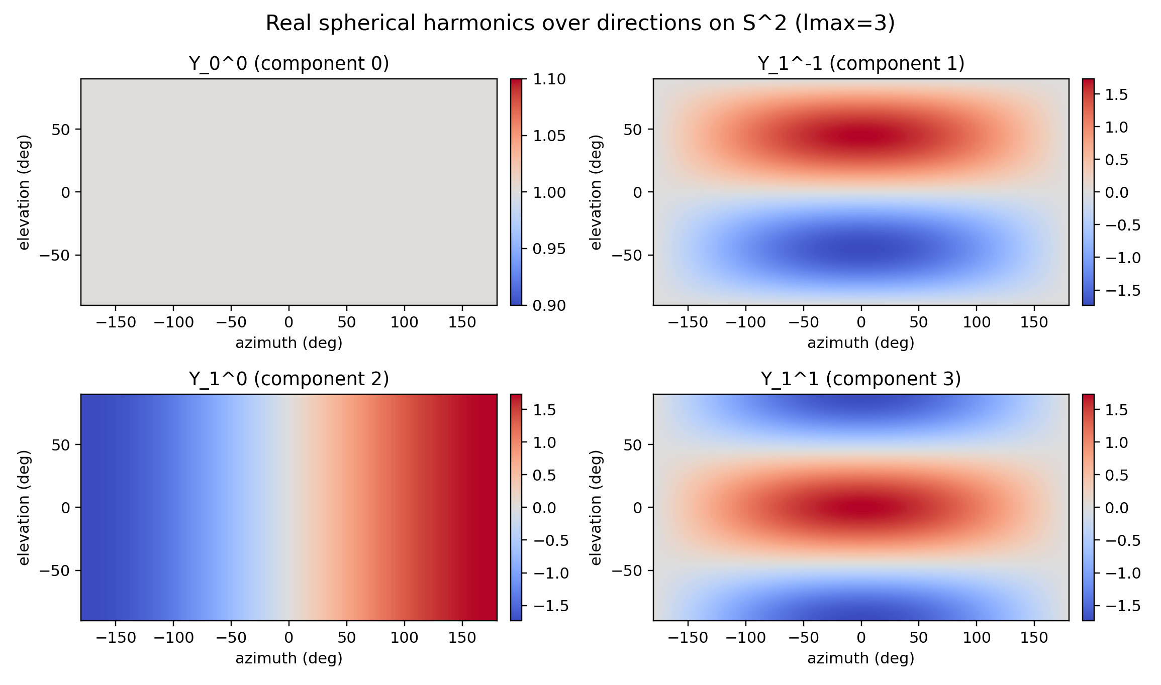
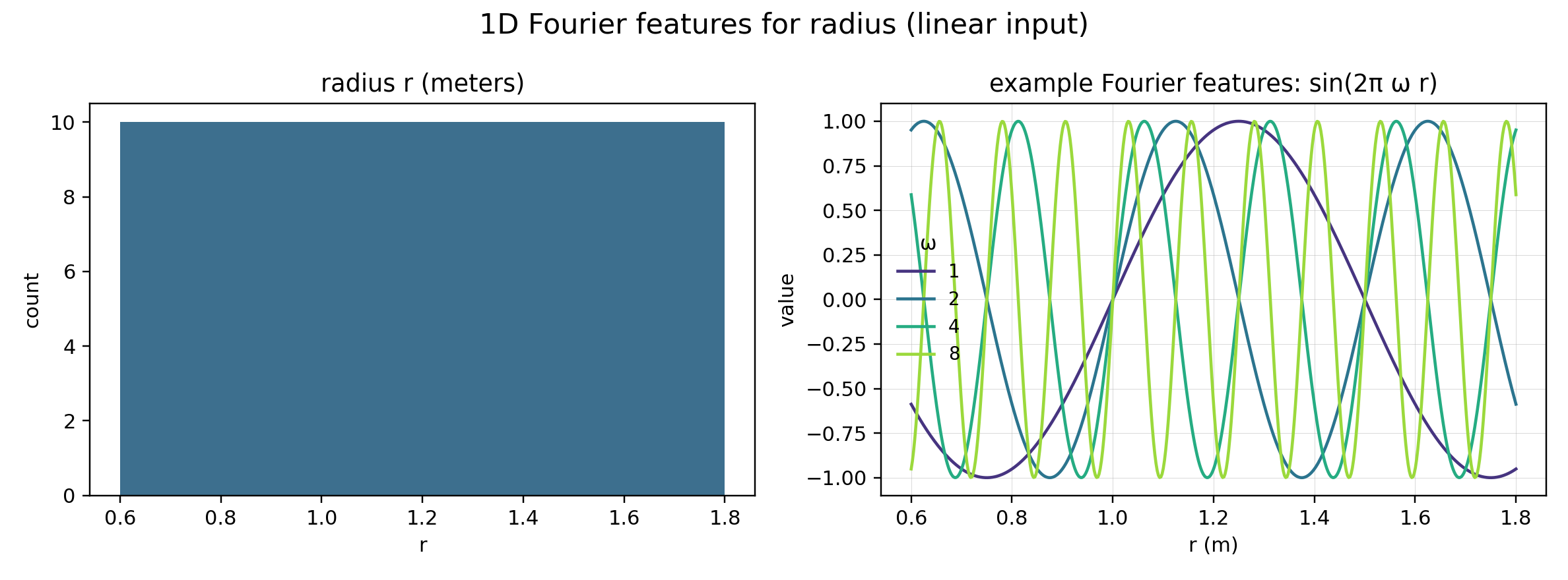
Actual encoding plots generated with `oracle_rri.vin.plotting.build_vin_encoding_figures` using the legacy
`ShellShPoseEncoderConfig` (lmax=2, 6 frequencies, linear radius input) on a sample snippet.
:::
## Legacy output dimensionality (default)
With defaults (`16` dims each for $u,f,r,s$) we get:
$$
\text{pose\_enc}(u,f,r,s)\in\mathbb{R}^{64}.
$$
# VIN head (v0.1 architecture)
`oracle_rri/oracle_rri/vin/model.py` (`VinModel`) implements a lightweight scorer head on top of a frozen EVL backbone:
1. Run frozen EVL once on the snippet to get low-dimensional head/evidence volumes + voxel grid pose (`EvlBackbone`).
2. Build a **voxel-aligned scene field** with `scene_field_channels` (default: `["occ_pr", "occ_input", "counts_norm"]`).
3. Project the field with a **1×1×1 Conv3d + GroupNorm + GELU** (default: `C_in=3 → field_dim=16`).
4. Compute a **global context token** via pose-conditioned attention pooling over a coarse voxel grid
(optional; `use_global_pool=True`, `global_pool_mode="attn"` by default; mean/mean+max are available).
5. Encode the **voxel grid pose** (`voxel/T_world_voxel`) in the *reference rig frame* using the same
`LearnableFourierFeatures` pose encoder. This is a global token shared by all candidates
(`use_voxel_pose_encoding=True` by default).
6. For each candidate:
- pose token: `LearnableFourierFeatures([u,f,r,s])` → `pose_enc` (default: 64 dims),
- local token: sample **K = grid_size² × len(depths)** frustum points in world coordinates (default: `4²×4=64`),
sample the voxel field there, then pool with an **unknown-token mean** (or masked mean) → `local_feat` (default: 16 dims).
7. Concatenate `[pose_enc, global_feat?, voxel_pose_enc?, local_feat, valid_frac?]` and score with
`VinScorerHead` (MLP + CORAL logits). `valid_frac` exposes frustum coverage so low-coverage candidates can still
score highly when they reveal unknown surfaces.
# VIN head (v0.2 simplified architecture)
`oracle_rri/oracle_rri/vin/model_v2.py` (`VinModelV2`) keeps only the most promising components and removes
architecture toggles while exposing a **configurable pose encoder** via a discriminated union.
1. **Pose encoding (reference frame, configurable).**
We compute the relative pose
$T_{\text{rig}\leftarrow\text{cam}} = T_{\text{world}\leftarrow\text{rig}}^{-1} T_{\text{world}\leftarrow\text{cam}}$
and then encode it with the selected pose encoder:
- **Default (`r6d_lff`)**: $x=[t/s_t,\; \mathrm{r6d}(R)/s_r] \in \mathbb{R}^9$, where $\mathrm{r6d}$ is the 6D
rotation representation (first two columns of $R$) [@zhou2019continuity]. The per-group scales $(s_t,s_r)$ are
**learned** to balance translation vs. rotation before the LFF encoder (see PyTorch3D transforms
[@pytorch3d-transforms]).
- **Optional (`shell_lff`, `shell_sh`)**: shell descriptors $(u,f,r,s)$ with forward direction only. These ignore
roll about the forward axis, which is acceptable when roll jitter is small; use `r6d_lff` if roll matters.
2. **Scene field (configurable channels).**
The current implementation constructs a compact field from EVL heads/evidence and then projects it with
`1×1×1 Conv3d + GroupNorm + GELU`. The **implemented** channels are:
- `occ_pr`, `cent_pr`, `occ_input`, `counts_norm`,
- `observed`, `unknown`, `free_input`, `new_surface_prior`.
The default `scene_field_channels` list is
`["occ_pr", "occ_input", "counts_norm", "cent_pr", "free_input", "new_surface_prior"]`.
3. **Global context (pose-conditioned attention).**
A coarse voxel grid is pooled and attended by the pose embeddings. Keys are augmented with an **LFF positional
encoding over XYZ voxel centers** derived from `voxel/pts_world` (normalized voxel coordinates) before attention.
The pooler now uses **separate keys and values**, plus a minimal **LayerNorm + residual + MLP** block for stability.
4. **View-dependent semidense features (official).**
For each candidate, we project semidense points into the candidate view and compute lightweight coverage/depth
statistics (coverage, empty fraction, valid fraction, depth mean/std). In addition, the same projected points
are summarized with **multi-head cross-attention (MHCA)** conditioned on the candidate pose, producing a
view‑specific frustum descriptor. Both signals are appended to the head input and provide explicit VIN‑NBV‑style
view conditioning.
5. **Optional semidense point encoder (PointNeXt‑S).**
A snippet‑level semidense embedding can be computed once and repeated for all candidates. This is useful as a
global scene prior but is not view‑specific; it is therefore treated as an auxiliary signal. When enabled, the
embedding can modulate `global_feat` via a FiLM‑style scale/shift
(feature‑wise linear modulation [@FiLM-perez2018]) — currently an experimental option.
6. **Optional trajectory context.**
If enabled, a trajectory encoder summarizes the snippet’s rig poses and appends the context to each candidate.
7. **CORAL head.**
We concatenate `[pose_enc, global_feat, semidense_proj, semidense_frustum, semidense_feat?, traj_ctx?]` and
score with the CORAL head.
8. **Frame correction (cw90).**
If candidates/poses were rotated by `rotate_yaw_cw90` in the labeler, the model **undoes** the rotation on
the input poses (no camera rebuild is needed in v2).
**Pose conditioning pathways.** In v2, pose information reaches the head along two paths:
- **Direct**: `pose_enc` is concatenated into the final feature vector.
- **Contextual**: `pose_enc` is also used as the query for pose‑conditioned attention over the voxel field.
This makes the model robust to early attention instability while still enabling view‑aware global context.
## Known issues / improvement targets (VIN v2)
- **Candidate-relative positional encoding**: global attention still uses absolute voxel positions in the
reference rig frame. Relative encodings often help in 3D attention; consider switching to candidate‑relative
positions (see Point Transformer [@point-transformer-zhao2021]).
- **Stage effects**: VIN‑NBV uses stage‑normalized binning to handle early vs late reconstruction phases
[@VIN-NBV-frahm2025]. Adding a stage proxy scalar (e.g., mean coverage or point count) is a low‑cost improvement.
## Semidense projection features (current)
`VinModelV2` computes per‑candidate projection features from semidense points using the candidate cameras. The
feature vector is:
- `coverage`: fraction of pixels hit by at least one point,
- `empty_frac`: `1 - coverage`,
- `valid_frac`: fraction of projected points that fall inside the image bounds,
- `depth_mean`, `depth_std`: depth statistics of valid projected points.
These features are concatenated into the head input and act as an explicit view‑conditioning signal, similar in
spirit to VIN‑NBV’s projection‑based view descriptors.
## Semidense frustum MHCA (current)
`VinModelV2` also summarizes the **projected semidense points** with a lightweight
multi‑head cross‑attention (MHCA) block, using candidate pose embeddings as queries.
The token features are built from normalized screen coordinates, depth, and (optionally)
inverse distance standard deviation. This yields a **view‑specific frustum descriptor**
that complements the scalar projection statistics and injects a stronger inductive bias
for “what lies in front of the candidate.”
This block is optional and gated by `VinModelV2Config.enable_semidense_frustum` (default: `False`).
## Suggested upgrade roadmap (summary)
1. **(Done)** Key/value separation + residual/LN around the pose‑conditioned attention block.
2. **(Done)** View‑conditioned point features via semidense projection + MHCA frustum summary.
3. **Add a stage proxy scalar** (e.g., coverage mean, max counts, or point count) to the head input.
4. **Switch positional encoding to candidate‑relative** coordinates for attention keys.
5. **Optionally add voxel‑frustum local evidence** (sample a small K‑point frustum and pool).
6. **Optionally add candidate view‑plane feature grids** (VIN‑NBV‑style projection + CNN head).
## VIN internal architecture (current, with tensor shapes)
Shapes below match the current `VinLightningModule.summarize_vin()` output for a typical oracle batch with `B=1`,
`N=32` candidates, EVL voxel grid resolution `48³`, and VIN defaults. The v2 head does **not** use voxel‑frustum
sampling; instead, it includes **semidense projection features** per candidate
(`SEMIDENSE_PROJ_DIM=5`: coverage, empty fraction, valid fraction, depth mean/std) plus an optional **semidense frustum MHCA**
summary (`field_dim` channels, when enabled), and optional snippet‑level semidense/trajectory context embeddings.
```{mermaid}
flowchart TD
    subgraph In["Inputs"]
        efm["EFM snippet dict<br/>(unbatched: T×...)"]
        cand["candidate_poses_world_cam<br/>PoseTW(B,N,12)<br/>(example: 1×32×12)"]
        ref["reference_pose_world_rig<br/>PoseTW(B,12)"]
        p3d["p3d_cameras<br/>PerspectiveCameras(B*N)"]
    end

    subgraph Frozen["Frozen EVL backbone"]
        evl["EvlBackbone.forward(efm)"]
        out["EvlBackboneOutput<br/>occ_pr/cent_pr/occ_input/counts<br/>T_world_voxel, voxel_extent, pts_world"]
    end

    subgraph VIN["Trainable VIN v2 head"]
        field_in["scene_field<br/>field_in: (B,C_in,D,H,W)"]
        proj["field_proj<br/>1×1×1 Conv3d + GN + GELU"]
        pos["pos_grid from pts_world<br/>rig frame + LFF"]
        gpool["pose-conditioned attention<br/>global_feat: (B,N,C)"]

        rel["relative pose<br/>T_rig_ref_cam = T_world_rig_ref^{-1} T_world_cam"]
        poseenc["pose_enc (R6D+LFF or shell)<br/>pose_enc: (B,N,E_pose)"]

        semproj["semidense projection<br/>coverage/empty/valid/depth stats<br/>semidense_proj: (B,N,5)"]
        semfrustum["optional semidense frustum MHCA<br/>frustum_feat: (B,N,C)"]
        semfeat["optional PointNeXt-S<br/>semidense_feat: (B,C_point)"]
        traj["optional trajectory ctx<br/>traj_ctx: (B,C_traj)"]
        film["optional FiLM on global_feat"]

        concat["concat feats<br/>[pose_enc, global_feat, semidense_proj,<br/> semidense_frustum?, semidense_feat?, traj_ctx?]"]
        head["MLP + CORAL<br/>logits: (B,N,K-1)"]
    end

    efm --> evl --> out
    out --> field_in --> proj --> gpool --> concat
    out --> pos --> gpool
    ref --> rel
    cand --> rel --> poseenc --> gpool
    poseenc --> concat
    p3d --> semproj --> concat
    p3d --> semfrustum --> concat
    semfeat --> film --> gpool
    semproj --> film
    traj --> concat
    concat --> head
```
## Scene field construction (math, current)
`VinModel` builds a compact voxel-aligned tensor field $F(\mathbf{v})\in\mathbb{R}^{C_\text{in}}$ from EVL outputs
(`_build_scene_field(...)` in `oracle_rri/oracle_rri/vin/model.py`). With default channels:
- occupancy prior: $F_1=\text{occ\_pr}(\mathbf{v})\in[0,1]$,
- occupied evidence: $F_2=\text{occ\_input}(\mathbf{v})\in\{0,1\}$,
- coverage: $F_3=\text{counts\_norm}(\mathbf{v})\in[0,1]$ (see formula above).
For ablations/variants we also support:
- `observed`: $\mathbb{1}[\text{counts}>0]$,
- `unknown`: $1-\mathbb{1}[\text{counts}>0]$,
- `new_surface_prior`: $(1-\mathbb{1}[\text{counts}>0])\cdot \text{occ\_pr}$,
- `free_input`: EVL free-space evidence if available; otherwise a weak proxy derived from `counts` and `occ_input`.
The field is projected to `field_dim` channels (default `16`) by a 1×1×1 convolution + GroupNorm + GELU.
### Scene field construction in VinModelV2 (current)
`VinModelV2` builds an aux map in `_build_field_bundle` with the following keys:
- `occ_pr`, `cent_pr`, `occ_input`, `counts_norm`,
- `observed`, `unknown`, `free_input`, `new_surface_prior`.
All of these keys are supported in `scene_field_channels`; invalid entries now raise a
clear error during field construction.
## Candidate-conditioned voxel query (implemented)
We implement a **frustum point query** that is intentionally aligned with our depth renderer:
### 1) Sampling query points in front of the camera
We choose a small image-plane grid (`frustum_grid_size=g`) and a list of metric depths
`frustum_depths_m=[d_1,\dots,d_M]`. This gives $K=g^2M$ query points per candidate.
The points are constructed in the **same NDC convention** used by the depth backprojection code and unprojected via
PyTorch3D `PerspectiveCameras.unproject_points(..., from_ndc=True, world_coordinates=True)` (see
[PyTorch3D :: Cameras](https://pytorch3d.readthedocs.io/en/latest/modules/renderer/cameras.html) [@PyTorch3D-Cameras-2025]).
Practical note: our helper follows the “screen-space → NDC” mapping used by the renderer/backprojector (including the
sign convention +X left, +Y up).
### 2) Mapping world points into the EVL voxel grid
EVL provides the voxel grid pose $T_{\text{world}\leftarrow\text{voxel}}$ and its metric extent
`voxel_extent=[x_min,x_max,y_min,y_max,z_min,z_max]` in the voxel frame.
We invert the pose and transform the frustum points:
$$
\mathbf{p}_\text{voxel} = T_{\text{voxel}\leftarrow\text{world}}\,\mathbf{p}_\text{world},
\qquad
T_{\text{voxel}\leftarrow\text{world}} = T_{\text{world}\leftarrow\text{voxel}}^{-1}.
$$
Then we map metric voxel coordinates to **voxel-index coordinates** (per axis):
$$
i_x = \frac{x-x_{\min}}{\Delta x},\quad
i_y = \frac{y-y_{\min}}{\Delta y},\quad
i_z = \frac{z-z_{\min}}{\Delta z},
$$
with $(\Delta x,\Delta y,\Delta z)=\left(\frac{x_{\max}-x_{\min}}{W},\frac{y_{\max}-y_{\min}}{H},\frac{z_{\max}-z_{\min}}{D}\right)$.
This corresponds exactly to `efm3d.utils.voxel_sampling.pc_to_vox`. The actual trilinear sampling is delegated to
`efm3d.utils.voxel_sampling.sample_voxels` (internally `torch.nn.functional.grid_sample`, `align_corners=False`,
`padding_mode="border"`). ([GitHub][4])
### 3) Pooling and candidate validity
We sample the projected scene field at those voxel-index coordinates, producing frustum tokens
`tokens (B,N,K,C_out)` and a boolean in-bounds mask `token_valid (B,N,K)`.
We then compute the candidate-local token via a masked mean:
$$
\text{local\_feat}=\frac{\sum_k \mathbb{1}[\text{valid}_k]\;\mathbf{t}_k}{\sum_k \mathbb{1}[\text{valid}_k] + \varepsilon}.
$$
Candidate validity is derived from the **fraction** of frustum samples that fall inside the voxel grid, controlled by
`VinModelConfig.candidate_min_valid_frac` (default: 0.2) so we avoid admitting candidates with only a handful of
in-bounds samples.
# Training objective (VIN-NBV style): CORAL ordinal regression
VIN-NBV reports that directly regressing RRI is difficult; it discretizes RRI into ordinal bins and trains with CORAL.
We follow the same structure:
1. **Oracle labels**: for each snippet, generate candidates and compute oracle RRI using `OracleRriLabeler` (candidate → render depth → backproject PCs → mesh distance → RRI).
2. **Binning (current implementation)**: convert oracle RRI values to ordinal labels $y\in\{0,\dots,K-1\}$ using
`oracle_rri/oracle_rri/vin/rri_binning.py` (`RriOrdinalBinner`).
We fit $K-1$ **empirical quantiles** (equal-mass bins) on a stream of oracle RRIs and store the edges
$\mathbf{e}=(e_1,\dots,e_{K-1})$.
**Implementation details (`RriOrdinalBinner.fit_from_iterable`)**:
- Accumulates RRI chunks on CPU; ignores non-finite values.
- Computes quantiles at $q_j = j/K$ via `torch.quantile`.
- If edges collapse (duplicate quantiles), falls back to uniform edges between
the observed min/max (or `[-1,1]` as a last resort).
- Supports resumable fitting by saving `.pt` fit data and exporting the final binner as JSON.
Then for an RRI value $r$ the label is computed via `torch.bucketize`:
$$
y(r)=\sum_{j=1}^{K-1}\mathbb{1}[r \ge e_j].
$$
Practical notes:
- Fit data can be saved/resumed (`.pt` state with RRI chunks) and the fitted binner is saved as JSON (`num_classes`,
`edges`, optional `bin_means`, `bin_stds`, and `bin_counts` for priors).
- On training start, if `VinLightningModuleConfig.num_classes` differs from the saved binner JSON, the binner is
automatically refit and the JSON is overwritten with the new class count.
- If quantile edges collapse (degenerate quantiles), we fall back to uniform edges between the observed min/max (or
`[-1,1]` as a last resort).
3. **Loss (CORAL)**: we use CORAL (*Rank consistent ordinal regression*, see
[arXiv :: 1901.07884](https://arxiv.org/abs/1901.07884) [@CORAL-cao2019] and
[coral-pytorch](https://raschka-research-group.github.io/coral-pytorch/) [@coral-pytorch-2025]).
CORAL represents a K-class ordinal label $y\in\{0,\dots,K-1\}$ via $K-1$ binary “levels”:
$$
\text{level}_k(y)=\mathbb{1}[y>k],\qquad k=0,\dots,K-2,
$$
and predicts logits $\ell_k$ for each threshold. The loss is the sum of binary cross-entropies over thresholds
(see `oracle_rri/oracle_rri/vin/coral.py`).
Explicitly:
$$
\\mathcal{L}_{\\text{CORAL}}
=\\sum_{k=0}^{K-2}
\\left[-\\text{level}_k\\log\\sigma(\\ell_k)
-(1-\\text{level}_k)\\log(1-\\sigma(\\ell_k))\\right].
$$
**Random-classifier baseline.** If logits are zero (uninformative classifier), then
$p_k=\sigma(\ell_k)=0.5$ for all thresholds. The BCE for each level is $\log 2$,
so the expected CORAL loss is:
$$
\mathbb{E}[\mathcal{L}_{\text{CORAL}}]
=(K-1)\log 2.
$$
For our default $K=15$, this gives $14\log 2 \approx 9.70$, which is a useful sanity
check when interpreting training curves. The Lightning module logs
`coral_loss_rel_random = coral_loss / ((K-1)\log 2)` alongside the raw loss, plus
a candidate-level `top3_accuracy` metric for ordinal classification.
**Optional imbalance mitigation.** Threshold labels are imbalanced by construction (early thresholds have
many positives). We therefore support optional reweighting in `VinLightningModuleConfig`:
- `coral_bias_init="prior_logits"` initializes CORAL threshold biases from empirical priors (`bin_counts`),
instead of a generic descending scheme.
- `coral_loss_variant="balanced_bce"` applies per-threshold positive-class weighting using
$P(y>k)$ (from the fitted binner or the current batch).
- `coral_loss_variant="focal"` applies focal weighting to the per-threshold BCE to combat collapse
under severe imbalance [@FocalLoss-lin2017].
4. **Binning diagnostics (plots).** The script `oracle_rri/scripts/plot_vin_binning.py`
generates the RRI histogram with quantile edges and a dedicated edge plot (Seaborn):
::: {#fig-vin-rri-binning layout-nrow=2}
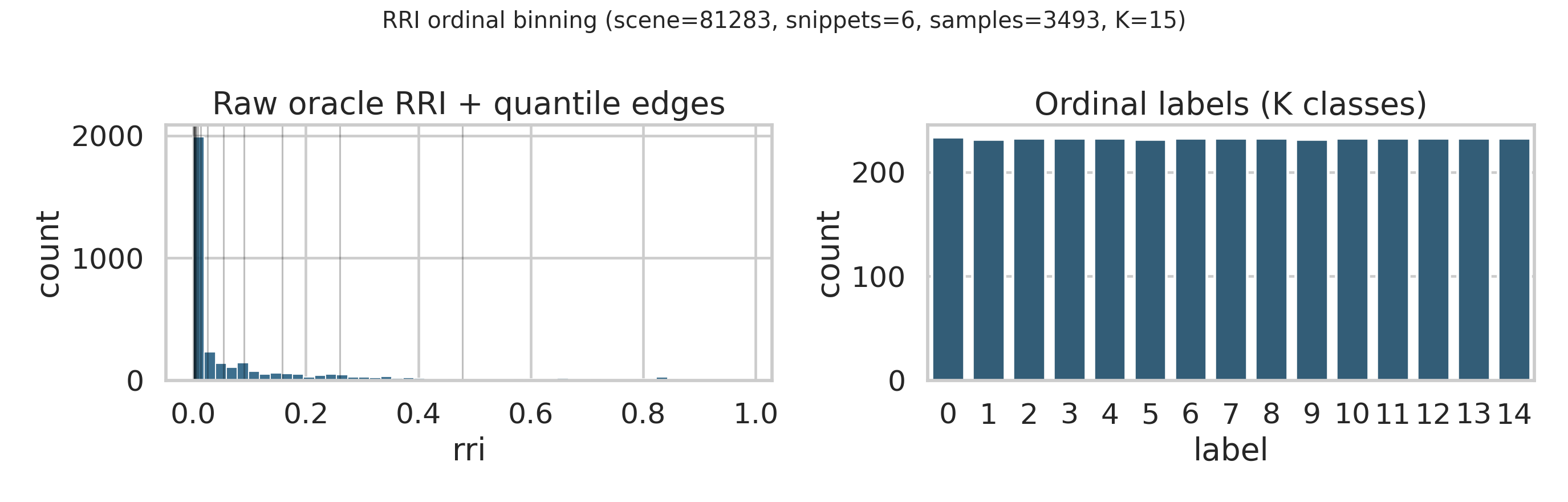
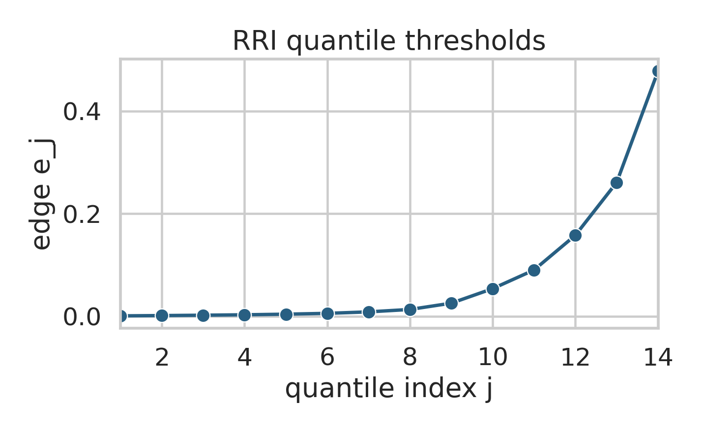
:::
At inference time we use the expected ordinal value (normalized to $[0,1]$) as the candidate score. With
$p_k=\sigma(\ell_k)=\mathbb{P}(y>k)$:
$$
\mathbb{E}[y]=\sum_{k=0}^{K-2} p_k,\qquad \mathbb{E}[y]_\text{norm}=\frac{\mathbb{E}[y]}{K-1}.
$$
# Minimal training script
End-to-end training/evaluation lives in the Lightning experiment stack (`oracle_rri/oracle_rri/lightning/`), exposed as
the console script `nbv-train` (see `oracle_rri/pyproject.toml`). Convenience wrappers exist in `oracle_rri/scripts/`
(e.g. `summarize_vin.py`, `train_vin_lightning.py`).
The pipeline does:
- load a real ASE snippet (local ATEK shards + meshes),
- run `OracleRriLabeler` online to produce labels,
- fit a binner (few snippets),
- train the head (EVL frozen) for a small number of steps.
Example:
```bash
cd oracle_rri
uv run nbv-train --run-mode summarize-vin
uv run nbv-train --run-mode plot-vin-encodings
uv run nbv-train --run-mode train
```
# Implementation map
VIN code lives in `oracle_rri/oracle_rri/vin/`:
- `backbone_evl.py`: `EvlBackbone` wrapper that consumes raw EFM dicts and returns a small typed `EvlBackboneOutput` (head outputs by default; optional neck outputs for ablations).
- `pose_encoding.py`: `LearnableFourierFeatures` (default; learnable Fourier + MLP over $[u,f,r,s]$).
- `pose_encoders.py`: pose-encoder variants for VIN v2 (discriminated union config, R6D LFF or shell-based LFF/SH).
- `spherical_encoding.py`: `ShellShPoseEncoder` (legacy; e3nn SH for $u,f$ + 1D Fourier for radius).
- `pose_encoding.py`: Learnable Fourier features baseline modules (as per Learnable Fourier Features, NeurIPS 2021).
- `model.py`: `VinModel` (pose encoding + scene-field querying + pose-conditioned global pooling + frustum sampling + CORAL).
- `coral.py`: CORAL layer + loss and probability utilities (via `coral-pytorch`).
- `rri_binning.py`: RRI→ordinal binning (`RriOrdinalBinner`).
# Known gaps / next steps (tracked in `todos.qmd`)
- add ranking metrics (Spearman, top-$k$ recall) to the training loop,
- version bin thresholds by candidate generator config + EVL ckpt id,
- run ablations: occ-only vs occ+obb, $L=2$ vs $L=3$, query depths/rays.


